Background and comparison

This article is the statistical background for the package, and a comparison against base R’s fisher.test() and exact2x2::fisher.exact(). The full derivations are in van der Meulen, Raymond and van der Meulen (2021), building on van der Meulen (2008).

Why a modified test

Fisher’s Exact Test fixes the total number of successes and asks only how they split between the groups; under the null that split is non-central hypergeometric with the odds ratio as its parameter. It never exceeds its nominal level α, but because the data are discrete it cannot in general hit size α exactly, so it ends up conservative: its true rejection rate sits below α, and a conservative test is underpowered.

Take a worked example with two independent binomial proportions \(u/m\) and \(v/n\), testing \(H_0: \theta = 1\) where \(\theta\) is the log odds ratio. Given \(u=13\), \(m=41\), \(v=6\), and \(n=47\) (Example 2 from the paper), the probability distribution for \(u\) is given by:

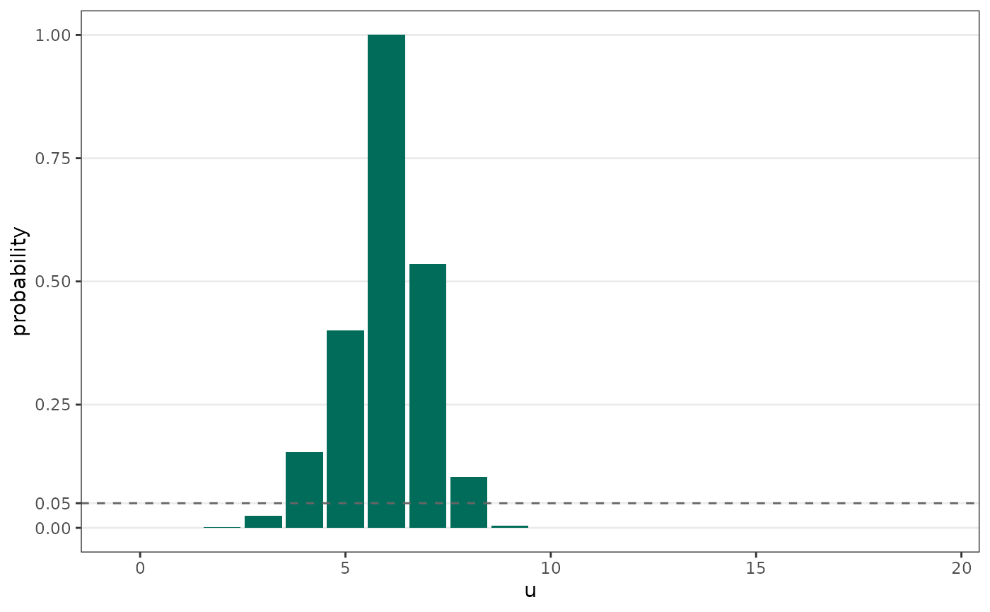
Fisher’s Exact Test is only uniformly most powerful unbiased (UMPU) if it is allowed to randomise at the borderline outcomes (e.g. randomising between \(u=\{3,4\}\) and \(u=\{8,9\}\)), in effect flipping a weighted coin to decide significance. That is rarely acceptable in practice, so a non-randomised version is used instead. The non-randomised tests all try to recover the power lost to dropping the coin flip, and differ in how, and in whether they still strictly control the Type I error rate:

The conservative / probability-based test rejects on the summed probability of outcomes at least as likely as the one observed. This is the “exact” test in SAS Proc FREQ and base R’s fisher.test(). It controls the size but is conservative, and its p-value and confidence interval can disagree (shown below).
Asymptotic tests (Woolf’s) and mid-p approaches are less conservative but do not strictly control the size; the true size can be larger than α.

The modified Fisher exact test in this package keeps strict size control while staying closest to the randomised UMPU test. It rejects at a borderline outcome only when its randomisation probability exceeds a single threshold γ₀, chosen to be as large as possible while keeping the maximum size (over the nuisance parameter) at or below α. Its p-value and confidence interval are test-based, so they agree by construction. The Overview of algorithm article shows how this is implemented.

The probability-based tests in R and SAS

The probability-based tests are familiar to many practitioners.

The two-sided p-value uses a likelihood ordering: it sums the probabilities of all tables no more likely than the observed one. Base R’s fisher.test() and SAS Proc FREQ use this same rule (in exact2x2 it is tsmethod = "minlike"), and it is the test implemented here as pvalue_probability().

Its confidence interval is calculated using a different method. fisher.test() does not invert that p-value; it uses an equal-tail (central) construction instead, the same mismatch holds for Proc FREQ. Because the two come from different rules, they can disagree: a result can be significant by its p-value while its interval still contains an odds ratio of 1.

Two further points concern the odds-ratio estimate, not the test. fisher.test() reports the conditional maximum likelihood estimate, whereas this package (following the paper) reports the sample odds ratio, so the estimates differ on identical data. And exact2x2::fisher.exact() lets you pick the two-sided method and pairs it with the matching interval: with tsmethod = "minlike" the interval inverts the same p-value, so the two agree - making it a suitable conservative comparator to modifiedfisher.

Side-by-side comparison

We use the paper’s Example 2: 13 of 41 in Group A versus 6 of 47 in Group B, testing the null odds ratio of 1 at α = 0.05.

Test	OR est.	p-value	CI lower	CI upper	OR = 1 in CI?
Modified FE (this package)	3.173	0.034	1.082	10.249	no
fisher.test() (base R)	3.130	0.039	0.969	11.312	yes
fisher.exact() minlike (exact2x2)	3.130	0.039	1.038	9.581	no
fisher.exact() central (exact2x2)	3.130	0.058	0.969	11.312	yes

Two things stand out:

The odds-ratio estimates differ, because fisher.test() and fisher.exact() report the conditional MLE while the modified test reports the sample odds ratio.
The last two columns, read together, show the disagreement between p-values and confidence intervals: base R’s fisher.test() can return a p-value below 0.05 while its 95% interval still contains an odds ratio of 1, because p-value and interval use different rules. The central variant makes the equal-tail interval (and its larger matching p-value) explicit; the minlike variant pairs the likelihood-ordering p-value with an agreeing interval. The modified test, like the agreeing exact2x2 options, never points its p-value and interval in opposite directions.

Which test controls what

Strict size control here means the actual size never exceeds α for any nuisance parameter value.

Test	Strict size control?	Non-randomised?	p-value and CI agree?	OR estimate
Randomised FE (UMPU)	yes (size = α exactly)	no	not usable	conditional MLE
Conservative / probability-based (base fisher.test, Proc FREQ)	yes (but conservative)	yes	no	conditional MLE
exact2x2 fisher.exact, minlike	yes (but conservative)	yes	yes	conditional MLE
Woolf asymptotic	no (can exceed α)	yes	yes	sample OR
Modified FE (this package)	yes (close to α)	yes	yes	sample OR

The randomised test is optimal but unusable in practice. The probability-based test is reproducible and controls the size, but is conservative and can give a disagreeing p-value and interval. Woolf’s test is self-consistent and cheap but does not strictly control the size. The modified test is the only row that is non-randomised, strictly size-controlling, and agreeing at once, which is what suits it to small-sample work needing strict Type I error control. The size and power of these tests are compared across the nuisance parameter in Reproducing the paper’s figures.

Unconditional exact tests

The tests compared above (Fisher’s, Woolf’s, and the modified test) are all conditional: they fix the total number of successes \(T = u + v\) and evaluate the extremity of the observed split.

A separate class of unconditional exact tests does not condition on \(T\). These fix only the sample sizes \(m\) and \(n\) and work with the full sample space of all possible \((u, v)\) pairs. Two key tests in this class are Barnard’s and Boschloo’s tests.

The power advantage of unconditional tests over the modified Fisher exact test is largest when only the sample sizes \(m\) and \(n\) are fixed by design (the typical setting in a randomised trial), since conditioning on \(T\) in that setting restricts the sample space without a design-based justification. The modified test’s advantage over the standard Fisher test holds within the conditional framework.

References

This ‘modified’ Fisher exact test:

van der Meulen EA, Raymond K, van der Meulen PJ (2021). Consistent Confidence Limits, P Values, and Power of the Non-Conservative, Size-α Modified Fisher Exact Test. Journal of Biostatistics and Biometric Applications 6(1):102.

van der Meulen EA (2008). A Nonrandomized, Nonconservative Version of the Fisher Exact Test. Communications in Statistics - Theory and Methods, 37:699-708.

The exact2x2 package is a useful resource for comparison tests: