
Reproducing the paper's figures
Comparing the size and power of the modified test against alternatives with the use of helper functions
Source:vignettes/articles/reproducing-paper-figures.Rmd
reproducing-paper-figures.RmdThis article rebuilds the size and power figures of van der Meulen, Raymond and van der Meulen (2021) from package functions alone, and the same helpers defined here can be pointed at your own design. For an overview of the function’s algorithm, see the Overview of algorithm article.
The size is maximised over the nuisance parameter \(\pi_1\) at every grid point, so larger sample sizes are slow. For that reason, the code and plots below use coarse grids by default; increase this grid to match a specific figure more closely.
Helpers
Construct size curves
Size is a function of the nuisance parameter \(\pi_1\). The helper evaluates all four tests over a grid of \(\pi_1\) for given sample sizes and null odds ratio, returning a data frame of size percentages. It needs the optimal \(\gamma_0\) first. Note that the conservative test is the modified test with \(\gamma_0 = 1\) (i.e. no boundary outcome ever rejected).
compute_size_curves <- function(m, n, alpha = 0.05, or = 1, precision = 1e-3,
                                p0_grid = seq(0.05, 0.95, by = 0.05),
                                method = "zoom", maze = 10, zoom_iter = 6) {

  df <- construct_test_frame(.odds_ratio = or, .m = m, .n = n,
                             .alpha = alpha, .precision = precision)

  gamma0_opt <- optimise_gamma0(.odds_ratio = or, .m = m, .n = n,
                                .alpha = alpha, .precision = precision,
                                .method = method, .maze = maze,
                                .zoom_iter = zoom_iter, .df = df)

  # Rejection matrices depend only on (df, gamma0), not on p0: build each
  # once and evaluate the whole p0_grid in a single batched call, rather than
  # rebuilding the matrix and re-deriving dbinom() vectors at every point.
  R_modified     <- modifiedfisher:::.build_rejection_matrix(df, gamma0_opt, m, n)
  R_conservative <- modifiedfisher:::.build_rejection_matrix(df, 1, m, n)

  data.frame(
    p0 = p0_grid,
    modified = modifiedfisher:::.local_size_modified_grid(
      p0_grid, .odds_ratio = or, .m = m, .n = n,
      .rejection_matrix = R_modified) * 100,
    woolf = sapply(p0_grid, function(p)
      local_size_asymptotic(p, .odds_ratio = or, .m = m, .n = n,
                            .alpha = alpha) * 100),
    sas_freq = sapply(p0_grid, function(p)
      local_size_probability(p, .odds_ratio = or, .m = m, .n = n,
                             .alpha = alpha) * 100),
    conservative = modifiedfisher:::.local_size_modified_grid(
      p0_grid, .odds_ratio = or, .m = m, .n = n,
      .rejection_matrix = R_conservative) * 100
  )
}
Construct power curves
Power is a function of the two response rates \(\pi_1\) and \(\pi_2\). Holding \(\pi_1\) fixed, the helper sweeps \(\pi_2\) and returns each test’s power as a percentage. The modified and conservative tests reuse the same test frame and \(\gamma_0\) as above.
compute_power_curves <- function(m, n, pi1 = 0.2, alpha = 0.05, or = 1,
                                 precision = 1e-3,
                                 pi2_grid = seq(0.25, 0.6, by = 0.025),
                                 method = "zoom", maze = 10, zoom_iter = 6) {

  df <- construct_test_frame(.odds_ratio = or, .m = m, .n = n,
                             .alpha = alpha, .precision = precision)

  gamma0_opt <- optimise_gamma0(.odds_ratio = or, .m = m, .n = n,
                                .alpha = alpha, .precision = precision,
                                .method = method, .maze = maze,
                                .zoom_iter = zoom_iter, .df = df)

  R_modified <- modifiedfisher:::.build_rejection_matrix(df, gamma0_opt, m, n)

  data.frame(
    pi2 = pi2_grid,
    modified = modifiedfisher:::.power_modified_grid(
      pi1, pi2_grid, .odds_ratio = or, .m = m, .n = n,
      .rejection_matrix = R_modified, .superiority = FALSE) * 100,
    woolf = sapply(pi2_grid, function(pi2)
      power_asymptotic(c(pi1, pi2), .m = m, .n = n, .alpha = alpha) * 100),
    sas_freq = sapply(pi2_grid, function(pi2)
      power_probability(c(pi1, pi2), .m = m, .n = n, .alpha = alpha) * 100),
    conservative = sapply(pi2_grid, function(pi2)
      power_conservative(c(pi1, pi2), .m = m, .n = n, .df = df,
                         .alpha = alpha, .precision = precision,
                         .superiority = FALSE) * 100)
  )
}
Define shared plotting style
Both figures share a colour and line-type scheme, with the nominal level α drawn as a dashed reference line on the size plot.
test_levels <- c("Modified", "SAS PROC Freq", "Woolf", "Conservative")

test_cols <- c(
  "Modified"      = "#016c59",
  "SAS PROC Freq" = "#3690c0",
  "Woolf"         = "#67a9cf",
  "Conservative"  = "grey70"
)

test_lty <- c(
  "Modified"      = 1,
  "SAS PROC Freq" = 4,
  "Woolf"         = 2,
  "Conservative"  = 6
)

to_long <- function(df, value_col, key_col) {
  df |>
    pivot_longer(modified:conservative, names_to = "test",
                 values_to = value_col) |>
    mutate(test_label = factor(case_when(
      test == "modified"     ~ "Modified",
      test == "woolf"        ~ "Woolf",
      test == "sas_freq"     ~ "SAS PROC Freq",
      test == "conservative" ~ "Conservative"
    ), levels = test_levels))
}
Size figure
We use \(m = 27\), \(n = 21\) for the null \(\mathrm{OR} = 1\), which corresponds to Figure 2(a) in the paper. The modified test (solid) tracks just under the dashed α line across the whole range, while the conservative test sits well below it.
alpha <- 0.05
size_df <- compute_size_curves(m = 27, n = 21, alpha = alpha, or = 1)

size_long <- to_long(size_df, "size", "test")

ggplot(size_long, aes(p0, size, colour = test_label, linetype = test_label)) +
  geom_hline(yintercept = alpha * 100, linetype = 2, colour = "grey30") +
  geom_line(linewidth = 0.9) +
  scale_colour_manual(values = test_cols) +
  scale_linetype_manual(values = test_lty) +
  coord_cartesian(ylim = c(0, 1.1 * alpha * 100)) +
  labs(x = expression(pi[1]), y = "Size (%)",
       colour = NULL, linetype = NULL,
       title = "Size of the modified Fisher exact test",
       subtitle = "m = 27, n = 21, H0: OR = 1") +
  theme_bw() +
  theme(legend.position = "bottom")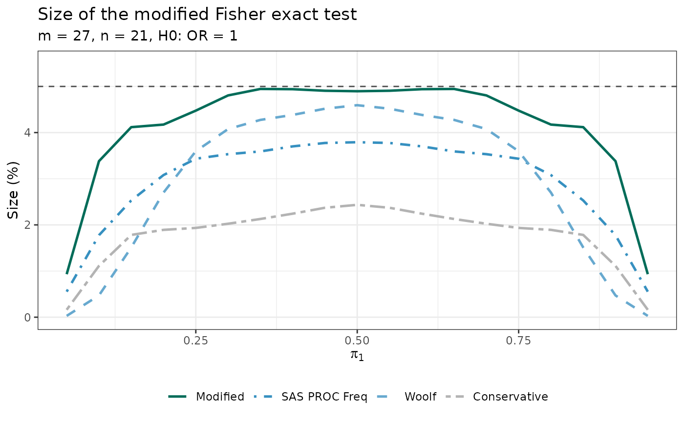
Power figure
For power we use \(m = n = 30\) with \(\pi_1 = 0.2\), matching the configuration of Figure 5(b). The modified test (solid) should sit at or above the probability-based test (the dashed comparator in the paper) across the alternative space.
power_df <- compute_power_curves(m = 30, n = 30, pi1 = 0.2, or = 1)

power_long <- to_long(power_df, "power", "test")

ggplot(power_long, aes(pi2, power, colour = test_label, linetype = test_label)) +
  geom_line(linewidth = 0.9) +
  scale_colour_manual(values = test_cols) +
  scale_linetype_manual(values = test_lty) +
  labs(x = expression(pi[2]), y = "Power (%)",
       colour = NULL, linetype = NULL,
       title = "Power of the modified Fisher exact test",
       subtitle = "m = n = 30, pi1 = 0.2, H0: OR = 1") +
  theme_bw() +
  theme(legend.position = "bottom")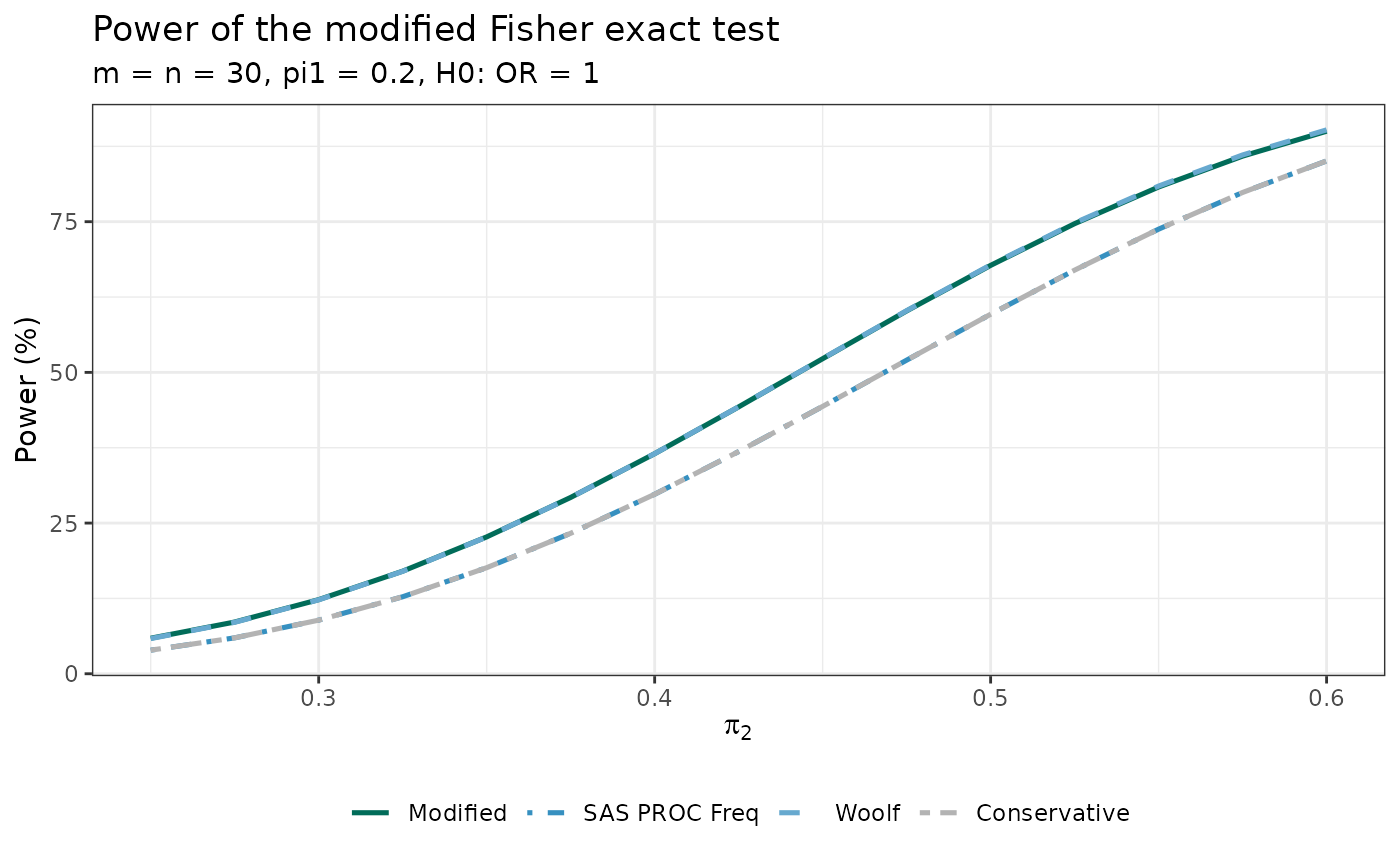
Matching a specific figure
To reproduce a paper figure exactly, set m and
n to that figure’s values, use a fine grid (the paper steps
\(\pi_1\) in 0.01), and for the OR = 2
panels pass or = 2 to both helpers. For example, Figure
3(a) is m = 65, n = 71,
or = 1.
Speed gain over the SAS macro
The original paper reports CPU times of roughly a minute at \(N = 50\) rising to an hour at \(N = 300\), mainly because the size is re-maximised over the nuisance parameter at every grid point in the SAS macro.
As of v0.0.4 of this package, the R function, using these same values, takes:
- roughly 1-2 seconds when \(N = 20\)
(i.e.
p0_grid = seq(1/20, 19/20, by = 1/20)), - roughly 4 seconds when \(N = 50\),
- roughly 8 seconds when \(N = 100\), and
- roughly 24 seconds when \(N = 300\),
measured on a moderately powerful laptop CPU (Apple M3 Pro).
The speed gain over the SAS macro comes primarily from the rejection
matrix built in .build_rejection_matrix(): instead of
re-evaluating the rejection rule for every table \((u, T)\) at each \(\pi_1\) grid point, the R implementation
builds the \((m+1) \times (n+1)\)
matrix \(R\) once per \(\gamma_0\) candidate and evaluates the
local size at any \(\pi_1\) as the
bilinear form \(p_u^\top R\, p_v\) (a
single matrix-vector multiplication).
Most of this package’s own internal speedups (v0.0.4) aren’t visible
above, since compute_size_curves() also computes the Woolf
and SAS Proc FREQ comparator sizes at every grid point, and neither was
part of that work. The SAS Proc FREQ comparator in particular recomputes
the full conditional hypergeometric distribution for every table and
dominates the total time shown here regardless of how fast the modified
test’s own calculation is.
# Figure 3(a) of the paper (slow):
size_fig3a <- compute_size_curves(
  m = 65, n = 71, or = 1,
  p0_grid = seq(1/100, 99/100, by = 1/100)
)

# Calculate time taken in R:
# microbenchmark::microbenchmark(compute_size_curves(m = 65, n = 71, or = 1, p0_grid = seq(1/20, 19/20, by = 1/20)), times = 10)
For context, the modified_fisher_exact_test() call
itself (with u = 13, m = 41,
v = 6, n = 47, and odds_ratio = 1
from Table 2 Example 2) takes 2.9 seconds.
Errors in Table 2
Two typos were identified in Table 2 of van der Meulen, Raymond and
van der Meulen (2021) while verifying the package against the worked
examples. The modifiedfisher package produces the correct
numbers in both cases.
Example 1 (5/12 vs 7/11): lower confidence limits are missing a leading zero. The correct lower limit for the modified test is 0.0716, not the printed 0.716 (and likewise 0.076 not 0.760 for Woolf, and 0.055 not 0.550 for Proc FREQ). The misprint is also self-contradictory: a test-based interval of (0.716, 2.210) cannot exclude its own point estimate of 0.408.
Example 4: the success count for Group A should be \(u = 71\), not 72. The heading “72/128 vs 58/142” is incorrect. With \(u = 71\), the estimate (1.804), p-value (0.0175), and confidence interval (1.108, 2.936) all match the printed values exactly; with \(u = 72\) none of them do.
Examples 2 and 3 are correct as printed. Both typos were confirmed
using closed-form Woolf limits and base R’s fisher.test(),
neither of which relies on any package code.