Get started

The non-conservative, size-$\alpha$ modified Fisher exact test rejects the null at a critical value only when the corresponding randomisation probability exceeds a threshold $\gamma_0$, chosen so the test’s size (maximised over the nuisance parameter) is as large as possible without exceeding $\alpha$.

This makes it less conservative than the standard Fisher exact test while still strictly controlling the Type I error rate. For why this matters and how it compares to other tests, see the Background and comparison article; for how it is built, see Overview of algorithm.

This vignette is a tour of modified_fisher_exact_test(), using the worked examples from van der Meulen, Raymond and van der Meulen (2021).

Basic usage

The test compares two independent binomial proportions $u/m$ and $v/n$, testing $H_0: \theta = \theta_0$ where $\theta$ is the log odds ratio. By default odds_ratio = 1 (equality of proportions).

We reproduce Example 2 from the paper’s Table 2: 13 of 41 versus 6 of 47.

library(modifiedfisher)
result <- modified_fisher_exact_test(u = 13, m = 41, v = 6, n = 47,
                                     odds_ratio = 1, local_size_data = TRUE)
result
#> 
#>  Non-Conservative Size-α Modified Fisher's Exact Test
#> 
#> data:  u = 13, v = 6, m = 41, n = 47
#> p-value = 0.03369
#> alternative hypothesis: true odds ratio is not equal to 1
#> 95 percent confidence interval:
#>   1.082336 10.249348
#> sample estimates:
#> odds ratio 
#>   3.172619

The result is an htest, so the usual components are available directly, and they match Table 2 (odds ratio 3.173, p-value 0.034, 95% CI 1.082 to 10.25):

result$estimate
#> odds ratio 
#>   3.172619
result$p.value
#> [1] 0.03369141
result$conf.int
#> [1]  1.082336 10.249348
#> attr(,"conf.level")
#> [1] 0.95

P-values and confidence intervals agree

Both are derived from the same test, so odds_ratio is rejected at level alpha if and only if it falls outside conf.int. The two can never disagree. This is not true of stats::fisher.test() or the SAS Proc FREQ exact test, whose p-values and intervals are built separately and can conflict. The Background and comparison article shows a worked case.

Scope and limitations

modified_fisher_exact_test() implements a two-sided test only. The null hypothesis is $H_0$: OR = odds_ratio, and the alternative is two-sided: OR $\neq$ odds_ratio. One-sided p-values and one-sided confidence bounds are not currently returned.

For superiority trials where the direction of the effect is specified in advance, the superiority = TRUE argument adjusts the power calculation to count only tables where the observed rate in group 2 exceeds that in group 1. This does not change the test or p-value; it narrows the power evaluation to the relevant region.

Formal one-sided inference (a one-sided p-value and a one-sided confidence bound) is outside the current scope of the package.

A different null hypothesis

The odds_ratio argument sets $\theta_0$; this does not need be 1. The estimate and confidence interval do not depend on it (only the p-value and $null.value change).

result_or2 <- modified_fisher_exact_test(u = 13, m = 41, v = 6, n = 47,
                                         odds_ratio = 2)
result_or2$p.value
#> [1] 0.4360352
result_or2$conf.int
#> [1]  1.082336 10.249348
#> attr(,"conf.level")
#> [1] 0.95

Precision and optimisation method

Two arguments control the numerics:

precision is the tolerance for the bisection searches behind the confidence limits and p-value (default 1e-3). A smaller value is more accurate but needs more size evaluations, which is the expensive step.
method selects how the size is maximised over the nuisance parameter. The default "zoom" refines a grid search and is usually fastest; "trust" uses a trust-region optimiser with an analytic gradient. They agree to within precision. For "zoom", maze sets the grid points per iteration and zoom_iter the number of refinements.

result_trust <- modified_fisher_exact_test(u = 13, m = 41, v = 6, n = 47,
                                           odds_ratio = 1, method = "trust")

result_trust$p.value
#> [1] 0.03369141

Power

The test also returns its power at two response rates power_at_pi1 and power_at_pi2 under the null odds_ratio used to build the test frame. This is the unconditional probability of rejecting $H_0$ at when $\pi_1=$power_at_pi1 and $\pi_2=$power_at_pi2. The default values are 0.5 and 0.75, respectively, but these can be changed:

result_power <- modified_fisher_exact_test(u = 13, m = 41, v = 6, n = 47,
                                           odds_ratio = 1, power_at_pi1 = 0.3,
                                           power_at_pi2 = 0.6)

result_power$power
#> [1] 80.40905

Set power = FALSE to skip this, which saves time for larger samples. Setting superiority = TRUE restricts the calculation to a positive observed effect (one-directional alternative), which (as the paper notes) only slightly changes power for relevant effect sizes:

result_sup <- modified_fisher_exact_test(u = 13, m = 41, v = 6, n = 47,
                                         odds_ratio = 1, power_at_pi1 = 0.3,
                                         power_at_pi2 = 0.6, superiority = TRUE)

result_sup$power
#> [1] 80.409

Sample size planning

The power functions can be inverted to answer the planning question: given a target power, what sample sizes are needed? There is no closed-form answer, so the simplest approach is a grid search over candidate values of $m$ and $n$.

The example below finds the smallest equal-allocation sample size ($m = n$) needed to achieve 80% power against $\pi_1 = 0.3$, $\pi_2 = 0.6$ under $H_0$: OR = 1 at $\alpha = 0.05$:

target_power <- 80   # percent
pi1 <- 0.3
pi2 <- 0.6
alpha <- 0.05
 
# Search over candidate n = m from 10 to 100
results <- data.frame(n = integer(), power = numeric())
 
for (n_candidate in 10:100) {
  
  df_candidate <- construct_test_frame(
    .odds_ratio = 1, .m = n_candidate, .n = n_candidate,
    .alpha = alpha, .precision = 1e-3
  )
  
  g0_candidate <- optimise_gamma0(
    .odds_ratio = 1, .m = n_candidate, .n = n_candidate,
    .alpha = alpha, .precision = 1e-3,
    .method = "zoom", .maze = 10, .zoom_iter = 6,
    .df = df_candidate
    )
  
  pwr <- power_modified(
    p          = c(pi1, pi2),
    .gamma0    = g0_candidate,
    .odds_ratio = 1,
    .m         = n_candidate,
    .n         = n_candidate,
    .df        = df_candidate,
    .alpha     = alpha,
    .precision = 1e-3,
    .superiority = FALSE
  )
  
  results <- rbind(results, data.frame(n = n_candidate, power = pwr * 100))
  
  # Stop when desired power is reached:
  if (pwr * 100 >= target_power) break
  
}
 
# Show last three rows:
tail(results, 3)
#>     n    power
#> 33 42 77.75243
#> 34 43 79.13426
#> 35 44 80.10992

The smallest $n$ achieving 80% power is 44 per group, giving 80.1% power. The search stops at the first $n$ that crosses the threshold; inspect results to see how power grows with sample size.

For unequal allocation, replace the loop with a grid over pairs $(m, n)$. Note that the power calculation re-runs the full test optimisation at each candidate sample size, so the search is slow for large candidate ranges. A coarse first pass (step size 5 or 10) followed by a fine search around the crossing point is more efficient.

Diagnostic: plotting the size

The size of the modified test is found numerically, so it is worth confirming the optimiser has not mistaken a local peak for the global one. local_size_data = TRUE attaches the local size at 101 values of the nuisance parameter $\pi_1$:

result$local.size.data |> head()
#>    pi1       size method
#> 1 0.00 0.00000000   zoom
#> 2 0.01 0.05426853   zoom
#> 3 0.02 0.46179445   zoom
#> 4 0.03 1.25223277   zoom
#> 5 0.04 2.16089076   zoom
#> 6 0.05 2.96284034   zoom

Plotting this data:

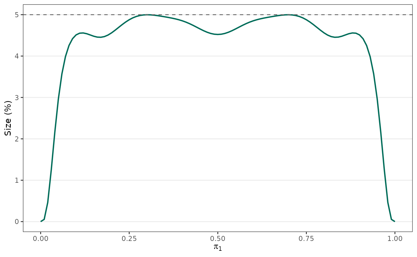
Local size of the modified Fisher exact test against the nuisance parameter, with a reference line at alpha.

The curve should stay at or below $\alpha \times 100\%$ throughout, touching it across a broad central region. This is the non-conservative behaviour behind the modified test’s power advantage.

Internals: gamma0 and the test frame

For advanced use or for checking against the original SAS/IML macro, the result exposes the threshold and the full test frame. $gamma0 is the optimal $\gamma_0$; $support.data holds, for every total $T$, the critical values $c_1, c_2$ and randomisation probabilities $\gamma_1, \gamma_2$.

result$gamma0
#> [1] 0.4950519
result$support.data |> head()
#>   t c1 d1    gamma1 c2 d2    gamma2
#> 1 0  0  0 0.0250000  0  1 0.0250000
#> 2 1  0  0 0.0500000  1  2 0.0500000
#> 3 2  0  0 0.0945652  2  3 0.1087500
#> 4 3  0  0 0.1807246  3  4 0.2398077
#> 5 4  0  0 0.3491271  4  4 0.5364119
#> 6 5  0  1 0.6554145  4  5 0.0428649

The boundary outcomes the modified test rejects (but the conservative test does not) are exactly those with a randomisation probability above the threshold:

result$support.data |> 
  filter(gamma1 > result$gamma0 | gamma2 > result$gamma0)
#>     t c1 d1    gamma1 c2 d2    gamma2
#> 1   4  0  0 0.3491271  4  4 0.5364119
#> 2   5  0  1 0.6554145  4  5 0.0428649
#> 3   7  1  1 0.2337006  6  6 0.6111712
#> 4   8  1  2 0.5169722  6  7 0.0852055
#> 5   9  1  2 0.9803533  7  8 0.4001280
#> 6  10  2  2 0.2198852  8  8 0.8747505
#> 7  11  2  3 0.5174349  8  9 0.2309683
#> 8  12  3  3 0.0072742  9  9 0.6657947
#> 9  14  3  4 0.6087134 10 10 0.4950519
#> 10 17  4  5 0.7890628 12 12 0.9331548
#> 11 19  5  6 0.5165288 13 13 0.8006534
#> 12 21  6  6 0.3163047 14 14 0.7126309
#> 13 22  6  7 0.7373777 14 15 0.1989687
#> 14 23  7  7 0.1586046 15 15 0.6565864
#> 15 24  7  8 0.5268783 15 16 0.1606163
#> 16 25  8  8 0.0283864 16 16 0.6253905
#> 17 27  8  9 0.8235340 17 17 0.5960512
#> 18 29  9 10 0.6356104 18 18 0.5778886
#> 19 31 10 11 0.4841665 19 19 0.5749891
#> 20 33 11 11 0.3592251 20 20 0.5863044
#> 21 34 11 12 0.8468401 20 21 0.1424674
#> 22 35 12 12 0.2544432 21 21 0.6113470
#> 23 36 12 13 0.7024766 21 22 0.1600169
#> 24 37 13 13 0.1656454 22 22 0.6501001
#> 25 38 13 14 0.5826859 22 23 0.1870078
#> 26 39 14 14 0.0900074 23 23 0.7029931
#> 27 41 15 15 0.0255816 24 24 0.7709303
#> 28 43 15 16 0.9406416 25 25 0.8491776
#> 29 45 16 17 0.8491776 26 26 0.9406416
#> 30 47 17 18 0.7709303 26 27 0.0255816
#> 31 49 18 19 0.7029931 27 28 0.0900074
#> 32 50 19 19 0.1870078 28 28 0.5826859
#> 33 51 19 20 0.6501001 28 29 0.1656454
#> 34 52 20 20 0.1600169 29 29 0.7024766
#> 35 53 20 21 0.6113470 29 30 0.2544432
#> 36 54 21 21 0.1424674 30 30 0.8468401
#> 37 55 21 22 0.5863044 30 30 0.3592251
#> 38 57 22 23 0.5749891 31 31 0.4841665
#> 39 59 23 24 0.5778886 32 32 0.6356104
#> 40 61 24 25 0.5960512 33 33 0.8235340
#> 41 63 25 26 0.6253905 33 34 0.0283864
#> 42 64 26 26 0.1606163 34 34 0.5268783
#> 43 65 26 27 0.6565864 34 35 0.1586046
#> 44 66 27 27 0.1989687 35 35 0.7373777
#> 45 67 27 28 0.7126309 35 35 0.3163047
#> 46 69 28 29 0.8006534 36 36 0.5165288
#> 47 71 29 30 0.9331548 37 37 0.7890628
#> 48 74 31 32 0.4950519 38 38 0.6087134
#> 49 76 32 33 0.6657947 38 39 0.0072742
#> 50 77 33 33 0.2309683 39 39 0.5174349
#> 51 78 33 34 0.8747505 39 39 0.2198852
#> 52 79 34 35 0.4001280 40 40 0.9803533
#> 53 80 35 35 0.0852055 40 40 0.5169722
#> 54 81 35 36 0.6111712 40 40 0.2337006
#> 55 83 37 37 0.0428649 41 41 0.6554145
#> 56 84 37 38 0.5364119 41 41 0.3491271

The mechanics of this are covered in Overview of algorithm, and the size and power of the comparison tests in Reproducing the paper’s figures.

References

van der Meulen EA, Raymond K, van der Meulen PJ (2021). Consistent Confidence Limits, P Values, and Power of the Non-Conservative, Size-$\alpha$ Modified Fisher Exact Test. Journal of Biostatistics and Biometric Applications, 6(1):102.

van der Meulen EA (2008). A Nonrandomized, Nonconservative Version of the Fisher Exact Test. Communications in Statistics - Theory and Methods, 37:699-708.

An overview of modifiedfisher and its options